Ecole des Mines de Nantes, 4 rue Alfred-Kastler, Nantes 44307, France
Institut de Recherches en Communications et en Cybernetique de Nantes, 1 rue de la Noe, 44321 Nantes, France
(Submmited to "IEEE Transactions on Robotics", 2011)
Previous page | Outline | Next page
Explicit expressions (13) derived in previous sections allow obtaining the Cartesian stiffness matrix instantly, for any Jacobian ![]() describing special location of the passive joints. However, recursive equation allows essentially simplify the computational procedure by sequential modification of the original stiffness matrix
describing special location of the passive joints. However, recursive equation allows essentially simplify the computational procedure by sequential modification of the original stiffness matrix ![]() for each passive joint independently, using separate columns of
for each passive joint independently, using separate columns of ![]() . Moreover, for some typical cases, relevant computations may be easily performed analytically. This section presents some useful techniques related to this approach.
. Moreover, for some typical cases, relevant computations may be easily performed analytically. This section presents some useful techniques related to this approach.
Let us assume that a current recursion deals with a single passive joint corresponding to the i-th column of the Jacobian ![]() , which is denoted as
, which is denoted as ![]() and has size
and has size![]() . In this case, the matrix expression
. In this case, the matrix expression ![]() is reduced to the size of
is reduced to the size of ![]() and the matrix inversion is replaced by a simple scalar division. Besides, the term
and the matrix inversion is replaced by a simple scalar division. Besides, the term ![]() has size
has size ![]() , so the recursion is simplified to
, so the recursion is simplified to
 |
(16) |
where ![]() is a
is a ![]() vector and
vector and ![]() is a scalar. Using methodology presented in Appendix A, it can be also proved that each recursions reduces the rank of the stiffness matrix by 1
is a scalar. Using methodology presented in Appendix A, it can be also proved that each recursions reduces the rank of the stiffness matrix by 1
(17) |
provided that the current Jacobian ![]() is independent of the previous ones
is independent of the previous ones ![]() (i.e. the i-th passive joints is not redundant relatively to the joints
(i.e. the i-th passive joints is not redundant relatively to the joints ![]() ).
).
Since in practice any combination of passive joints can be decomposed into elementary translational and rotational ones, it is enough to consider only two types of the Jacobian columns ![]() :
:
(18) |
where the unit vector ![]() ,
, ![]() defines orientation of the passive joint axis (both for translational and rotational ones) and the vector
defines orientation of the passive joint axis (both for translational and rotational ones) and the vector ![]() defines influence of the rotational passive joints on the linear velocity at the reference point, i.e.
defines influence of the rotational passive joints on the linear velocity at the reference point, i.e. ![]() where
where ![]() is a vector from the joint centre point to the reference point. After relevant substitutions, one can obtain the following expression for the translational joint
is a vector from the joint centre point to the reference point. After relevant substitutions, one can obtain the following expression for the translational joint
 |
(19) |
and for the rotational one
 |
(20) |
Hence, in general case, the recursion involves rather intricate matrix transformation, different from simple setting to zero a row and/or a column. Let us consider now several specific (but rather typical) cases where the transformation rules are more simple and elegant.
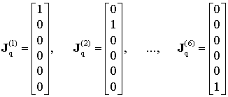
In practice, many parallel robots include kinematic chains for which the passive joint axes are collinear to the axes x, y or z of the Cartesian coordinate system. For such architectures, the vector-columns of the Jacobian ![]() include a number of zero elements, so the expressions (13) can be essentially simplified. Let us consider a set of trivial cases where
include a number of zero elements, so the expressions (13) can be essentially simplified. Let us consider a set of trivial cases where ![]() are created from the columns of the identity matrix
are created from the columns of the identity matrix ![]() :
:
 |
(21) |
Corresponding passive joints will be further referred to as the ‘trivial’ ones. It can be easily proved that they cover the following range of the joint geometry:
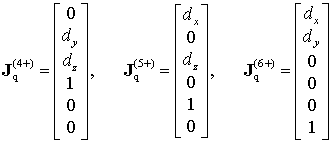
Besides, it is worth to consider additional case-study corresponding to
which will be further referred to as the ‘quasi-trivial’ and gives the Jacobian columns of the following structure:
 |
(22) |
where ![]() denote the elements of the vector
denote the elements of the vector ![]() , which are equal here either
, which are equal here either ![]() or 0.
or 0.
For the trivial passive joints, assuming that ![]() denotes the vector-column with a single non-zero element in the p-th position, a straightforward substitution yields
denotes the vector-column with a single non-zero element in the p-th position, a straightforward substitution yields ![]() ;
; ![]() . So, the recursive expression (16) for the Cartesian stiffness matrix is simplified to
. So, the recursive expression (16) for the Cartesian stiffness matrix is simplified to
 |
(23) |
that is very similar to those presented in the motivation example (see Section II). Also, here the p–th row and column of the matrix ![]() become equal to zero
become equal to zero
(24) |
and the recursive computations are easily performed analytically.
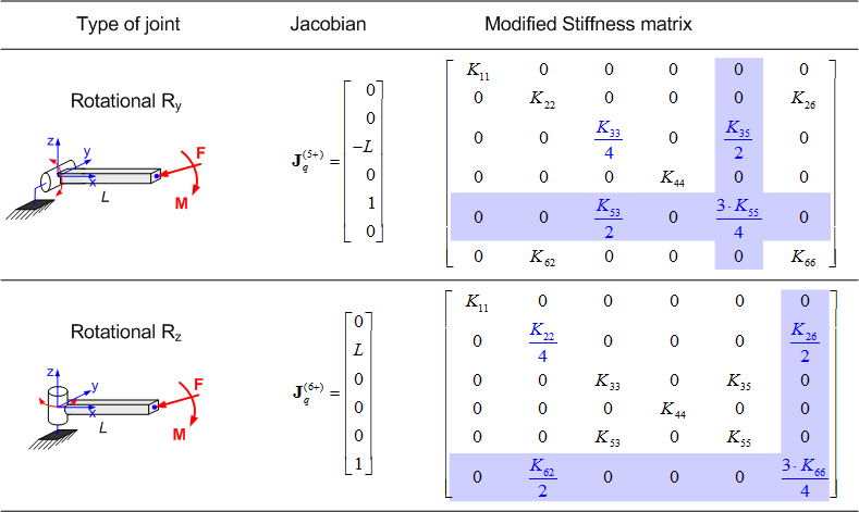
For practical convenience, the above considered case-studies are summarized in Table 2 where the original stiffness matrix
 |
(25) |
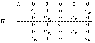
is assumed to be sparse in accordance with the structure corresponding to a beam-type link whose cross-section are symmetrical with respect to y- and z-axis, and its elements are expressed via the physical parameters as
 |
(26) |
where L is the link length, A is its cross-section area, Iy, Iz, and J are the quadratic and polar moments of inertia of the cross-section, and E and G are the Young’s and Coulomb’s modules respectively.
Table II
Stiffness matrix transformations caused by trivial passive joints
(for the case of original stiffness matrix (25))
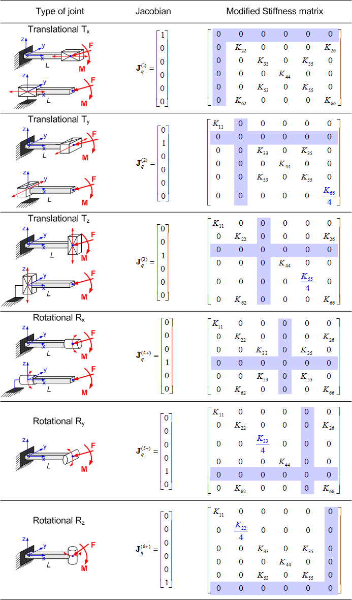
As follows from these results, trivial passive joints can be easily taken into account by using simple analytical expressions , but relevant modifications of the stiffness matrix are more serious than simple zeroing of relevant rows and columns (in addition, some elements must be reduced in half or fourfold, see Table 2). Moreover, for the quasi-trivial passive joints, the stiffness matrix may be singular but does not include purely zero rows and columns (see Table 3). Hence, the developed technique is essential for VJM-based stiffness modeling of mechanisms with passive joints.
Table III
Examples of stiffness matrix transformations for quasi-trivial passive joints
(for the case of original stiffness matrix (25))
